nextnano3 - Tutorial
next generation 3D nano device simulator
1D Tutorial
ISFET (Ion-Selective Field Effect Transistor): Electrolyte Gate AlGaN/GaN Field Effect Transistor as pH Sensor
Author:
Stefan Birner
If you want to obtain the input file that is used within this tutorial, please
submit a support ticket.
-> 1DGaN_electrolyte_sensor.in
This tutorial is based on the following paper
Theoretical
study of electrolyte gate AlGaN/GaN field effect transistors
M. Bayer, C. Uhl, P. Vogl
Journal of Applied Physics 97 (3), 033703, (2005)
as well as on the diploma theses of both Christian Uhl and Michael Bayer.
Note that this tutorial only briefly sketches the underlying physics. So
please check these references for more details.
Acknowledgement: The author - Stefan Birner - would like to thank
Christian Uhl and Michael Bayer for helping to include the electrolyte features into nextnano³.
Electrolyte Gate AlGaN/GaN Field Effect Transistor as pH Sensor
Here, we predict the sensitivity of electrolyte
gate AlGaN/GaN field effect transistors (FET) to pH values of the electrolyte
solution that covers the semiconductor structure. Particularly, we need to take
into account the piezo- and pyroelectric polarization fields according to the
pseudomorphic growth of the nitride heterostructure on a sapphire substrate
(However, here we assume that the heterostructure is strained with respect to
GaN).
The charge density due to chemical reactions at the oxidic
semiconductor-electrolyte interface is described within the site-binding model ($interface-states).
We calculate the spatial charge and potential distribution both in the
semiconductor and the electrolyte (Poisson-Boltzmann equation)
self-consistently.
The AlGaN/GaN FET that is exposed to an electrolyte solution has the
following schematic layout:
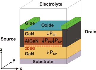
Fig. 1: AlGaN/GaN FET with electrolyte gate.
The polarization charges are included for the case of Ga-face polarity.
The polarization fields lead to the formation of a 2DEG.
We simulate the structure along the z direction
and neglect source and drain so that the structure is effectively
one-dimensional, i.e. laterally homogeneous.
The nitride heterostructure is assumed to be grown along the hexagonal [0001]
direction and is of Ga-face polarity. The AlGaN layer is strained with respect
to GaN but the remaining layers are unstrained.
The piezo- and pyroelectric polarization of wurtzite GaN and Al0.28Ga0.72N
result in huge polarization fields within the structure. The divergence of the
total polarization across the interface between adjacent layers causes a fixed
interfacial sheet charge density.
The following figure shows the influence of the interface charge densities:
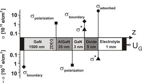
Fig. 2: Schematic layout of the calculated AlGaN/GaN heterostructure
including the interface charge densities. The magnitudes are indicated by the
filled symbols.
The file
densities/interface_densitiesD.txt gives us information about the
relevant interface charge densities:
- Interface 1 (1 nm): sigmaboundary = - 2.2 * 1013
e / cm²
as defined in the input file:
 $interface-states

  state-number         =
  1
   ! between Metal / GaN at 1 nm

  state-type           =
  fixed-charge !
  -sigma_boundary

  interface-density    = -2.2d13
   ! -2.2 x 10^13 [|e|/cm^2]
- Interface 2 (1500 nm): sigmapolarization (Interface 2) =
sigmapiezo + sigmapyro = 1.38 * 1013 e / cm²
-> sigmapiezo = 6.61 * 1012 e / cm²
-> sigmapyro = 7.14 * 1012 e / cm²
- Interface 3 (1535 nm): sigmapolarization (Interface 3)
= - sigmapolarization (Interface 2)
- Interface 4 (1538 nm): sigmaboundary as for Interface 1
(but with different sign) plus an additional charge sigma* = 1.0 * 1013
e / cm² as defined in the input file:
 $interface-states

  state-number         =
  3
   ! between GaN / Oxide at 1538 nm

  state-type           =
  fixed-charge ! sigma*

  interface-density    = 1.0d13
    ! 1 x 10^13 [|e|/cm^2]
- Interface 5 (1543 nm): sigma* as for Interface 4 (but with
different sign) plus an additional charge sigmaadsorbed that
results from the site-binding model that describes chemical reactions at the
oxidic semiconductor-electrolyte interface. More details:
$interface-states
 $interface-states

  state-number          =
  5
  ! between Oxide / Electrolyte at 1543 nm

  state-type
  = electrolyte !
  sigma_adsorbed

  interface-density     = 9.0d14
  ! [cm^-2] -
total
density of surface sites, i.e. surface hydroxyl groups
  adsorption-constant   = 1.0d-8
  ! K1 = adsorption   constant

  dissociation-constant = 1.0d-6
  ! K2 = dissociation constant


 $electrolyte

  ...

  pH-value
  = 5.3d0       !
pH = -lg(concentration) = 5.3 -> [M]=[mol/l]
For the origin of sigmaboundary and sigma* please refer to the
references that are given above.
The GaN region (1 nm - 1500 nm) is homogeneously n-type doped with a
concentration of 1 * 1016 cm-3.
The electrolyte region (1543 nm - 2999 nm) contains the following ions:
 !---------------------------------------------------------------------------!

 ! The electrolyte (NaCl, Hepes) contains four types of ions:

 !   1) 100 mM singly charged cations (Na+)

 !   2) 100 mM singly charged anions  (Cl-)

 !   3)  10 mM doubly charged cations (Hepes2+ solution)

 !   4)  20 mM singly charged anions  (Hepes-
 solution)

 !---------------------------------------------------------------------------!

 $electrolyte-ion-content


  ion-number        =
1
!
100 mM singly charged cations
  ion-valency       =
1d0            !
 Na+

  ion-concentration = 0.100d0
!
Input in units of: [M] = [mol/l] = 1d-3 [mol/cm³]
ion-region =
1543d0 2999d0 ! refers to region where
the electrolyte has to be applied to
  ion-number        =
2
!
  ion-valency       =
-1d0 ! Cl-
ion-concentration = 0.100d0
! Input in units of: [M] = [mol/l] = 1d-3 [mol/cm³]
ion-region =
1543d0 2999d0 ! refers to region where
the electrolyte has to be applied to
  ion-number        =
3
!
  ion-valency       =
2d0 ! Hepes2+
ion-concentration = 0.010d0
! Input in units of: [M] = [mol/l] = 1d-3 [mol/cm³]
ion-region =
1543d0 2999d0 ! refers to region where
the electrolyte has to be applied to
  ion-number        =
4
!
  ion-valency       =
-1d0 ! Hepes-
ion-concentration = 0.020d0
! Input in units of: [M] = [mol/l] = 1d-3 [mol/cm³]
ion-region =
1543d0 2999d0 ! refers to region where
the electrolyte has to be applied to
In addition to these four types of ions, the pH value (as specified in $interface-states)
automatically determines inside the code four further types of ions, namely the
concentration of H3O+, OH- and the
corresponding anions- (conjugate base: [anion-]
= 10-pH - 10-pOH = 10-5.3 - 10-8.7 =
5.01 x 10⁻⁶)
and cations+ (conjugate acid; zero in this tutorial because pH = 5.3
< 7). For
details, confer $electrolyte-ion-content.
We have to solve the nonlinear Poisson equation over the whole device, i.e.
including the Poisson-Boltzmann equation that governs the charge density in the
electrolyte region.
As for the boundary conditions we assume at the right boundary
(Electrolyte/Metal) a Dirichlet boundary condition where the electrostatic
potential phi is equal to UG where UG is the gate voltage
determined by an electrode in the electrolyte solution and which is constant
throughout the entire electrolyte region. In this example the applied gate
voltage is UG = 0 V. Note that the reference potential UG
enters the Poisson-Boltzmann equation and also the equation for the site-binding
model at the oxide/electrolyte interface. So the Dirichlet boundary condition is
phi = 0 V. This corresponds to the fact that at the right part of the
electrolyte, i.e. at 'infinity' (at 2999 nm) the ion concentration is the
'equilibrium' (default) concentration as defined in
$electrolyte-ion-content.
At the left boundary (Metal/GaN) we use a generalized Neumann boundary
condition with a potential gradient that corresponds to the polarization charge
-sigmaboundary = - 2.2 * 1013 e / cm². Thus the electric
field E is given by
E = d phi / d z = -sigmaboundary / (epsilon0
* epsilonr) * (-1) = - 3.977 * 108 V/m.
epsilonr = vacuum-permittivity (see $physical-constants)
epsilon0(GaN along [0001] axis) = 10.01
Note that the generalized Neumann boundary condition is automatically taken
into account as sigmaboundary is specified at the left contact. Thus
it is not necessary to specify the electric field of
-3.977d8 V/m.
$poisson-boundary-conditions

   poisson-cluster-number  = 1

   region-cluster-number   = 1

   boundary-condition-type = Neumann

 ! Not necessary:

 ! electric-field          =
-3.977d8 ! -3.977 * 108 [V/m]
,
corresponds to sigmaboundary = - 2.2 * 1013
[e/cm2] at the left boundary
 ! Specify this instead:

   electric-field
= 0d0      ! 0 [V/m]


   poisson-cluster-number  = 2

   region-cluster-number   = 7

   boundary-condition-type = Dirichlet

   potential
= 0d0      ! phi = 0 [V]
<=> UG = 0 [V]
Oxide/electrolyte interface potential as a function of pH value
The GaN heterostructure acts as a sensor via the semiconductor-electrolyte
interface potential that reflects sigmaadsorbed, the pH value and the
spatial dependence of the electrostatic potential in the solution as described
by the Poisson-Boltzmann theory.
Choosing flow-scheme = 30, several
calculations are performed while sweeping over the pH value from 0 to 12.
    pH-value
=
(value is overwritten internally in the program)
The file InterfacePotential_vs_pH1D.dat gives us the
information about the electrostatic potential at the oxide/electrolyte interface
for different pH values.
We performed these calculations three times where we varied the adsorption
and dissociation constants.
adsorption-constant   = 1.0d-8
  ! K1 = adsorption   constant
  (best fit to experiment)

  dissociation-constant = 1.0d-6
  ! K2 = dissociation constant
  (best fit to experiment)
adsorption-constant = 1.0d-10
! K1 = adsorption constant
dissociation-constant = 1.0d-10
! K2 = dissociation constantadsorption-constant = 1.0d-10
! K1 = adsorption constant
dissociation-constant = 1.0d6
! K2 = dissociation constant
The total
density of surface sites, i.e. surface hydroxyl groups, was taken to be the
same in all three cases:
    interface-density     = 9.0d14
! [cm^-2]
The surface potential is defined as the difference of the electrostatic
potential at the oxide/electrolyte interface and the reference potential UG
(Here: UG = 0 V).
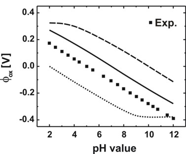
Fig. 3: Calculated oxide/electrolyte interface
potential as a function of the pH value.
The solid line shows the result for K1 = 10-8, K2
= 10-6.
Also included are the cases for K1 = 10-10, K2
= 10-10 (dashed line), K1 = 10-10, K2
= 106 (dotted line)
and the experimental data (G. Steinhoff et al., APL 83, 177 (2003).
Note that in Fig. 3 only the slope (d phi / d pH) is relevant but not the
absolute values of the potential. The experiment gives 56.0 +/- 0.5 mV/pH. Our
best fit parameters (solid line) yield 55.9 mV/pH and reproduce the constant
slope over the entire pH range.
Oxide/electrolyte interface charge density sigmaadsorbed as a
function of pH value
From the file InterfacePotentialDensity_vs_pH1D.dat we also obtain
information about the oxide/electrolyte interface sheet charge density sigmaadsorbed
(as a function of pH value) that is determined by the amphoteric reactions at
the oxide surface.
We plot in Fig. 4 for the following constants the oxide/electrolyte interface
charge density sigmaadsorbed:
  adsorption-constant   = 1.0d-8
! K1 = adsorption   constant
(best fit to experiment)

  dissociation-constant = 1.0d-6
! K2 = dissociation constant  (best
fit to experiment)
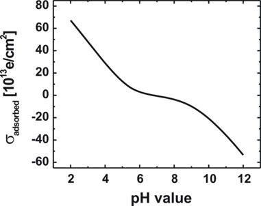
Fig. 4: Calculated variation of the
oxide/electrolyte interface charge density sigmaadsorbed of the
amphoteric oxide surface with the pH value of the electrolyte solution.
Note that there is a range of pH values where the net surface charge density is
close to zero.
The calculated point of zero charge for the GaO surface is reached for pH = 6.8.
Electrostatic potential for different electrolyte gate voltages UG
Now we want to plot the electrostatic potential for different values of UG,
i.e. for applying a gate voltage to the electrolyte. Note that UG is
both the Dirichlet boundary condition for the electrostatic potential at the
right contact as well as the reference potential that enters into the
Poisson-Boltzmann equation (i.e. into the exponential term of the ion charge
density).
UG is constant throughout the entire electrolyte region.
UG = 0.5 V:
   poisson-cluster-number  = 2

   region-cluster-number   = 7

   boundary-condition-type = Dirichlet

   potential
=  0.5d0    ! phi =  0.5 [V]
<=> UG =  0.5 [V]
UG = - 0.5 V:
   poisson-cluster-number  = 2

   region-cluster-number   = 7

   boundary-condition-type = Dirichlet

   potential
= -0.5d0    ! phi = -0.5 [V]
<=> UG = -0.5 [V]
The pH value is set to 5.3.
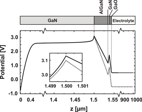
Fig. 5: Spatial electrostatic potential distribution for pH = 5.3 in the
electrolyte.
Depicted are the cases UG = 0.5 V (solid line) and UG = -
0.5 V (dotted line).
The inset illustrates the effect of an applied voltage on the potential near the
position of the 2DEG. |