|
Up
doping
generation
| | This is the old documentation.
Here's the link to the new documentation.
structure{}
Specifications that define the device structure. (New:
GDSII files
can be mapped onto region{...} using
nextnanopy.)
structure{
Output definitions
   output_region_index{
#
      boxes =
yes/no
#
   }
#
abrupt discontinuities at interfaces (in 2D four points, in 3D eight
points)
   output_material_index{
#
      boxes =
yes/no
#
   }

   output_contact_index{
#
      boxes =
yes/no             #
   }

   output_user_index{
#
      boxes =
yes/no
#
   }
#
#
# (i.e. regions without user index do not affect the user index array).
#
# And use variables together with expressions such as $index = $index + 1
to generate consecutive index values
from region to region.
#
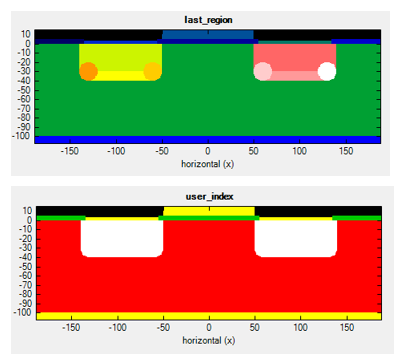
output_user_index_nnp.in

#
This example shows how to create an incremental enumeration of regions using variables,
and also how to keep identical number across clusters of regions.
   output_alloy_composition{
#
      boxes =
yes/no
#
   }

   output_impurities{
# [1018/cm3]
boxes =
yes/no
# (optional)
   }


output_generation{
# [10^18/(cm3
s)]
boxes = yes/no
# (optional)
}
Structure definitions
Every region needs to have a certain shape, which can be defined by
several objects.
It consists of a certain material and/or contact, and it can have a
doping profile.
Any subsequently defined region overwrites previously defined ones in the
overlapping area.
For exclusive properties such as material and contact, this implies a
substitution of the old value.
Concerning doping, the new profile is added to any previously defined
one.
Geometric objects may also be defined such that they are partially, mostly, or completely outside of the simulation region.
Only the parts of structures which are inside of the simulation region will be used, everything else is ignored.
The following structures are supported:
- 1D:
line
- 2D:
rectangle
circle
triangle
trapezoid
polygon
regular_polygon
hexagon
semiellipse
- 3D:
cuboid
sphere
cylinder
obelisk
hexagon_obelisk
cone
semiellipsoid
regular_prism
hexagonal_prism
polygonal_prism
pyramid
regular_pyramid
hexagonal_pyramid
polygonal_pyramid
region{
Region object
shapes
      user_index{
2 }
#
output_user_index{}.
# output_region_index{}.
When plotting, each region will be visualized with a different color.
# Sometimes the user wants to have the same color for several
regions, e.g. to set all regions that are doped to the same index. This can be
set here.
everywhere{}
# region will extend over the whole simulation area
#
# that should fill all "empty" (i.e. undefined) areas of the simulation
area.
      line{
#
         x =
[10.0, 20.0]
# 10
nm to 20
nm along the x direction
      }


      line{
#
         x =
[20.0, 10.0]
# 10
nm to 20
nm along the x direction, i.e. the reverse order x1 < x2
also works
      }


      rectangle{
#
         x =
[10.0, 20.0]
# 10
nm to 20
nm along the x direction
         y = [
0.0,  5.0]
# 0 nm to
5 nm along the y direction
      }


      cuboid{
#
         x =
[10.0, 20.0]
# 10
nm to 20
nm along the x direction
         y = [
0.0,  5.0]
# 0
nm to 5 nm along the y direction
         z = [
0.0,  5.0]
# 0 nm to
5 nm along the z direction
}
circle{ # 2D object, a circle is defined by its center and radius
         center{ x
= 10.5   y = 14.0
}           #
 regular_polygon

         radius =
10.0
             #
radius
}
      sphere{
#
3D object, a sphere is defined by its center and radius
         center{ x
= 10.5   y = 14.0
z = 1.0
} #
 circle

         radius =
10.0
             #
radius
}
cylinder{ # 3D object, e.g. a cylinder with a freely oriented axis
         axis_start =
[50.0, 50.0, 30.0]
#
         axis_end   =
[50.0, 50.0, 60.0]
#
         radius     =
20.0
   #
}
3D_Cylinder_nnp.in
      trapezoid{
#
2D object e.g. a simple trapezoid along the x axis
         base_x
= [ 5, 15]       #
5
to 15 nm
         base_y
= [25, 25]       #
25
nm
         top_x
= [ 8, 12]       #
8
to 12 nm
         top_y
= [30, 30]       #
30
nm
}
base_x and base_y has to be set by two equal numbers to
define the base line.
The same holds for top_x and top_y to define the top line.
      obelisk{
#
         base_x
= [ 5, 15]       #
         base_y
= [ 6, 17]       #
         base_z
= [27, 27]       #
         top_x
= [ 7, 13]       #
         top_y
= [ 8, 15]       #
         top_z
= [21, 21]       #
}
base_x, base_y, and base_z has to be set by two equal numbers to
define the base plane.
The same holds for top_x, top_y, top_z to define the top plane.
hexagon_obelisk{
# 3D object, an obelisk with its base and top planes
given by hexagons
... (same as obelisk
to define position, orientation and extension of object)
permute    = yes/no
#
(optional)
switch between two possible orientations of the hexagon
within the rectangularly defined planes
}
      semiellipse{
#
         base_x
= [45, 55]       #
         base_y
= [ 5,  5]
#
         top
= [50, 15]       #
50,15)
in units of [nm]
}
Note: Exactly one of
the elements base_x, and base_y has to be set by two equal numbers to define the
base line.
      semiellipsoid{
#
         base_x
= [25, 25]       #
         base_y
= [17,  6]
#
         base_z
= [ 7, 19]       #
         top
= [17, 13, 11] # 17,13,11)
in units of [nm]
}
Note: Exactly one of
the elements base_x, base_y, and base_z has to be set by two equal numbers to
define the base plane.
      cone{
#
         base_x
= [ 5, 20]       #
         base_y
= [20, 20]       #
         base_z
= [ 7, 19]       #
         top
= [10, 30, 11] # 10,30,11)
in units of [nm]
diminution =
0.0
# (optional) minimum value is 0.0
(i.e. cone),
maximum value is 1.0 (i.e. cylinder)
# diminution =
0.5
0.0 (i.e. cone)
}
base_x, base_y, and base_z has to be set by two equal numbers to
define the base plane.
      triangle{
#
2D object, a triangle defined by its
3 vertices.
         vertex{
x = 10.5   y = 14.0 } #
         vertex{
x =  0.0   y =  0.0 } #

         vertex{
x =  5.0   y =
10.0 } #

      }
      polygon{
#
2D object, a polygon defined by its vertices. If the first and the last
defined vertex are not identical, then they are joined with a line.
         vertex{
x = 10.5   y = 14.0 } #
#
}
      polygonal_prism{
#
3D object (= 2D polygon with
extension into the perpendicular direction; vertices define the circumference of the prism.)
         z = [0,
10]                   #
z direction.
vertex{
x = 10.5 y = 14.0
} #
a vertex P is defined by its x and y coordinates: P=(x,y). Multiple
vertices can and must be defined for a polygon.
#
         axis = [0,
1, 1]              #
# x, y,
z are possible.)
}
      regular_polygon{
#
2D object, a polygon with equal angles and equal side lengths. It is
defined by its center, one vertex and the number of facets.
         center{ x
= 10.5   y = 14.0
} #
         corner{ x
= 20.0   y = 30.0
} #
         number_of_facets =
7 # = number of vertices), must be >=
3
}
      regular_prism{
#
3D object (= 2D regular_polygon with
extension into the perpendicular direction; center and/or corner define the circumference of the prism.)
         z = [0,
10]                   #
z direction.
center{ x
= 10.5 y = 14.0
} #
The center point M is defined by its x and y coordinates: M=(x,y).
         corner{ x
= 20.0   y = 30.0
} #
         number_of_side_facets =
7 # = number of vertices), must be >=
3
axis = [0,
1, 1] #
(optional) inclination (shear) of prism structure
# x, y,
z are possible.)
}
      hexagon{
#
2D object, a polygon with equal angles and equal side lengths and 6
facets. It is defined by its center and one corner vertex.
         center{ x
= 10.5   y = 14.0
} #
 regular_polygon

         corner{ x
= 20.0   y = 30.0
} #
same as for regular_polygon
}
      hexagonal_prism{
#
3D object (= 2D hexagon with
extension into the perpendicular direction; center and/or corner define the circumference of the prism.)
         z = [0,
10]                   #
z direction.
center{ x
= 10.5 y = 14.0
} #
same as for regular_polygon
corner{ x
= 20.0 y = 30.0
} # same as for regular_polygon
axis = [0,
1, 1] #
(optional) inclination (shear) of prism structure
# x, y,
z are possible.)
}
Per default, all prisms (polygonal_prism, regular_prism, hexagonal_prism) are assumed to extend along the respective layer thickness direction (i.e. normal to the defining coordinate plane).
But, using the axis vector, an arbitrary axis (inclination) direction for the prism can be defined in the simulation system. The axis vector does not need to
be normalized, however, its orientation defines which side of the prism layer is the base to be used as reference for the inclination.
For example,
      regular_prism{


		      z = [50, -70]                              #
automatically reordered to [-70, 50]
center{ x =
10 y = 10 }
corner{ x =
30 y = 40 }
number_of_side_facets = 8 #
regular octagon wanted
			axis = [15 , 25 , 120]
 #
}
z
direction (end surfaces are x-y planes at z = -70
and z = +50).
Since the axis points upwards in z direction (z = 120), the base surface to be taken as reference is the lower x-y plane at z = -70.
There, the octagon center is at { x = 10
y = 10 } with an octagon corner at { x =
30 y = 40 }.
With the axis vector defined as above, we then find for the x-y plane at z =
+50
- the octagon center at { x = 10+15 y =
10+25} and
- the octagon corner at { x =
30+15 y =
40+25 }.
In analogy to polygon, we provide pyramidal structures.
      polygonal_pyramid{
#
3D object
      z = [70, -70]
#
 polygonal_prism

         vertex{
x = 10.5   y = 14.0
} #
a vertex P is defined by its x and y coordinates: P=(x,y). Multiple
vertices can and must be defined for a polygon.
#
         apex{   x =
10    y = 10   z =
120}


}


      regular_pyramid{
#
      z = [70, -70]
#
 regular_prism

         center{ x =
10    y = 10 }
#
same as for regular_prism
corner{ x =
70 y = 70 }
# same as for regular_prism
number_of_side_facets =
8 # same as for regular_prism
apex{ x =
10 y = 10 z =
120}
}
hexagonal_pyramid{
# 3D object
      z = [70, -70]
#
 hexagonal_prism

         center{ x =
10    y = 10 }
#
same as for hexagonal_prism
corner{ x =
70 y = 70 }
# same as for hexagonal_prism
apex{ x =
10 y = 10 z =
120}
}
Similar to the prismatic structures, use x, y, and
z at the beginning of the respective primitive to define the extent in the desired height direction, use vertex, center, and/or corner
to define the circumference of the base of the pyramid, and apex
to define the position of the apex of the pyramid.
Note that, for polygonal_pyramid (as for polygon), the vertices must be ordered either clockwise or counterclockwise, otherwise the behavior during structure generation will be undefined.
Also note that if the apex
is located outside of the interval defined by x, y,
or z at the beginning in the height direction, the pyramid will be truncated. Also, the pyramid will point upwards if the apex
is above the center of said interval (and the lower plane is used as base), and will point downwards if the apex
is below the center (and the upper plane is used as base). And in case a symmetric regular pyramid is desired, please make sure to laterally align the apex
with the center point.
For example
      regular_pyramid{


      z = [70, -70]

         center{ x =
10    y = 10 }

         corner{ x =
70   y = 70 }

         number_of_side_facets =
8

         apex{   x =
10    y = 10   z =
120}


}
defines a regular octahedral pyramid with base at z = -70, centered there at { x =
10 y = 10 }
and a corner there at { x = 70 y =
70 }.
The apex of the pyramid would be at { x = 10 y =
10 z = 120}, making the structure rotationally symmetric, except that the pyramid is truncated at z = +70.
Thus, a rotationally symmetric truncated octahedral pyramid has been defined.
pyramid{ #
3D object, e.g. a pyramid with 4 freely defined corner points
         point1 =
[50.0, 20.0, 30.0]
#
         point2 =
[50.0, 50.0, 80.0]
#
         point3 =
[80.0, 50.0, 50.0]
#
         point4 =
[50.0, 80.0, 30.0]
#
}
Contact
definition
      contact{
#
         name =
"source"
#
      }


      contact{
#
         name =
"source"
#

         remove{}
# contact
attribute,
# contact
attribute.
}
Depending on the dimension of the simulation domain, different options are available.
      binary{

         name    =
"GaAs"
#
      }


      ternary_constant{

         name    =
"Al(x)Ga(1-x)As"  #
         alloy_x =
0.2
# 0.0,
maximum value is 1.0)
      }


      ternary_linear{

         name    =
"In(x)Al(1-x)As"  #
         alloy_x =
[0.8, 0.2] # 0.0,
maximum value is 1.0)
         x
= [75.0, 125.0] # [nm]
y
= [10.0, 20.0] #
y coordinates of start and end point [nm] (2D
or 3D only)
         z
= [10.0, 20.0] # [nm] (3D only)
# (75,10,10)
to the point (125,20,20)
# and stays constant in the perpendicular planes.
}
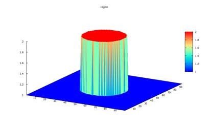
      ternary_pyramid{
#
(e.g. for InGaAs quantum dots) starting point and direction
(3D only)
         name    =
"In(x)Ga(1-x)As"  #
         alloy_x =
[0.28, 0.80] # cmincmax value of x content (minimum value is 0.0,
maximum value is 1.0)
#
#
         x
= [20.0, 0] # [nm]
y
= [20.0, 0] #
y coordinate of apex and y component of axis direction [nm]
z
= [11.0, 1] #
z coordinate of apex and z component of axis direction [nm]
# apex located at point (20.0,20.0,11.0)
(top of inverted
pyramid)
# 0,0,1),
i.e. along z axis
#
# i.e. (0,0,1)
will lead to the same pyramidal profile as (0,0,-1).
}
      c = cmin + ( cmax - cmin
) cos2(phi)
where phi is the angle to the
center axis. The formula is based on the model proposed by Tersoff (N. Liu et
al., PRL 84, 334 (2000)).
with high indium content for small
angles as indicated by the light regions in the figure shown below.
      ternary_trumpet{
#
(e.g. for InGaAs quantum dots) starting point and direction
(3D only)
         name    =
"In(x)Ga(1-x)As"  #
         alloy_x =
[0.2, 0.5] # cmincmax value of x content (minimum value is 0.0,
maximum value is 1.0)
         x
= [20.0, 0] # [nm]
y
= [20.0, 0] #
y coordinate of apex and y component of axis direction [nm]
z
= [11.0, 1] #
z coordinate of apex and z component of axis direction [nm]
# apex located at point (20.0,20.0,11.0)
(top of inverted
pyramid)
# 0,0,1),
i.e. along z axis
# The profile is symmetric with respect to the inverse of the direction
of the center axis,
# i.e. (0,0,1)
will lead to the same trumpet profile as (0,0,-1).
         z0
= 1.25
#
1e-10)
         rho0    =
0.6
#
1e-10)
}
      c = cmin + ( cmax - cmin
) exp [ ( - SQRT(x2 + y2) exp(-z1/z0) ) / rho0 ]
z0 and
rho0 can be used to vary the shape of the alloy profile while keeping the
average indium content fixed.
      ternary_import{

         name        =
"In(x)Al(1-x)As"          #
ternary material name for this region which uses imported alloy profile
         import_from =
"import_alloy_profile1D" # import{}. The imported
profile must have exactly one data component (x).
}
      quaternary_import{

         name        =
"Al(x)Ga(y)In(1-x-y)As"   #
quaternary material name for this region which uses imported alloy profile
         import_from =
"import_alloy_profile1D" # import{}. The imported
profile must have exactly two data components (x,y).
}
      quinternary_import{
...
#
analogous for quinternaries:
}
      quaternary_constant{

         name        =
"Al(x)Ga(y)In(1-x-y)As" #
quaternary
material name for this region with constant alloy profile
         alloy_x     =

0.2
# 0.0,
maximum value is 1.0)
         alloy_y     =
0.5
# 0.0,
maximum value is 1.0)
}
x + y <= 1
The interpolation of AxByC1-x-yH
is done according to eq. (E.10) in PhD thesis of T. Zibold apart from changes in
sign of bowing parameters.
The interpolation of AxB1-xCyD1-y
is done according to eq. (E.15) in PhD thesis of T. Zibold apart from changes in
sign of bowing parameters.
      quaternary_linear{

         name    =
"Al(x)Ga(y)In(1-x-y)As" #
quaternary
material name for this region with linear alloy profile
         alloy_x =
[0.2, 0.5]
# 0.0,
maximum value is 1.0)
         alloy_y =
[0.1, 0.3]
# 0.0,
maximum value is 1.0)
         x
= [20.0, 20.0]
# [nm]
y
= [20.0, 20.0]
# y
coordinates of start and end point [nm] (2D or 3D only)
         z
= [11.0, 20.0]
# [nm] (3D only)
      }


      quaternary_pyramid{
#
         name    =
"Al(x)Ga(y)In(1-x-y)As" #
         alloy_x =
[0.2, 0.5]
#
         alloy_y =
[0.1, 0.3]
#
         x
= [20.0, 0] # [nm]
y
= [20.0, 0] #
y coordinate of apex and y component of axis direction [nm]
z
= [11.0, 1] #
z coordinate of apex and z component of axis direction [nm]
# apex located at point (20.0,20.0,11.0)
(top of inverted
pyramid)
# 0,0,1),
i.e. along z axis
#
# i.e. (0,0,1)
will lead to the same pyramidal profile as (0,0,-1).
      }


      quaternary_trumpet{
#
         name    =
"Al(x)Ga(y)In(1-x-y)As" #
         alloy_x =
[0.2, 0.5]
#
         alloy_y =
[0.1, 0.3]
#
         x
= [20.0, 0] # [nm]
y
= [20.0, 0] #
y coordinate of apex and y component of axis direction [nm]
z
= [11.0, 1] #
z coordinate of apex and z component of axis direction [nm]
# apex located at
(20.0,20.0,11.0)
(top of inverted
pyramid)
# 0,0,1),
i.e. along z axis
#
# i.e. (0,0,1)
will lead to the same trumpet profile as (0,0,-1).
         z0
= 1.25
#
1e-10)
         rho0    =
0.6
#
1e-10)
}
      quinternary_constant{
... }
#
      quinternary_linear{
... }
#
      quinternary_pyramid{
... }
#
      quinternary_trumpet{
... }
#
      integrate{
#
electron_density{} #
hole_density{} #
piezo_density{} #
pyro_density{} #
polarization_density{} # ( = piezo + pyro)
label =
"channel"
# (optional) defines meaningful label for columns in
output files.
#
}
especially if
there is a significantly high density at the boundaries of the integration
region.
Doping profiles
       doping{

         ...

      }
Generation profiles
generation{

         ...

      }
Repeating regions
The following specifiers can be used to
define a periodically repeated pattern. Experimentally, a periodic geometry
might have been generated by e.g. etching.
This feature
is useful for multi-quantum wells, superlattices, Quantum Cascade Lasers, Bragg reflectors, etc.
Also, it is possible to make the number of layers a variable ($NUM_QUANTUM_WELLS) in a corresponding template.
Please also note to adjust the grid
accordingly (grid{}),
e.g. if a nonuniform grid is chosen.
Note:
array_x was previously called
repeat_x{} (and
max was called
num with
max=num-1).
repeat_x is deprecated and should be
replaced with array_x .
array_x{} copies
the region object. The loop runs from
-shift*min to
shift*max.
      array_x{
#
(optional)
shift
=
11.0 # repeat region in x direction by shifting it
11.0 nm (in units of [nm])
max
= 3 # shift 3
(=max) times (Here,
4 regions will be set: The original one, and 3
shifted ones.)
# max =
0
min
= 2 # 0)
repeat region in negative x direction 2
times, i.e. the region object will be
shifted 2
times by -shift.
# min =
0
# 2 (=min)
times into the negative direction and 3
(=max) times into the positive direction.
}
array_y{
# (optional, 2D and 3D only)
...
(same as
array_x but for y direction)
}
array_z{
# (optional, 3D only)
...
(same as
array_x but for z direction)
}
repeat_profiles
=
" #
enumerate profiles to be shifted. If repeat_profiles is not
defined, shift all profiles (default).
alloy #
doping #
generation # periodic
generation may be caused by having a periodic light absorbing mask
other #
" #
Example:
repeat_profiles =
"alloy generation"
If you want to shift
alloy/doping/generation profiles independent of each other you have to define
separate regions (region) for each,
for instance a separate region for doping where you add
array_x
and shift.
(==> region{ doping{...}
array_x{
shift = ... }})
For instance, two identical layers
containing 16 quantum dots each, can be easily generated by specifying only one quantum dot geometry.
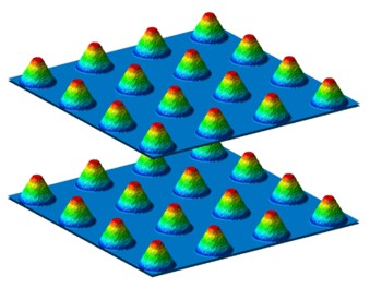
region{
cone{
# .
base_x
= [1.0,7.0] #
extension of base plane in x direction, i.e. from 1.0 to
7.0 nm
base_y
= [1.0,7.0] # 1.0 to
7.0 nm
base_z
= [6.0,6.0] #
top
= [4.0,4.0,10.0] # 4.0,4.0,10.0)
in units of [nm]
diminution =
0.25
# cone: diminution = 0.0,
cylinder: diminution = 1.0
}
Note:
Exactly one of the elements base_x, base_y, and base_z
has to be set by two
equal numbers to define the base plane.
ternary_linear{
name
=
"Al(x)Ga(1-x)As"
#
alloy_x =
[0.25, 1.0]
# x = 0.25 (Al0.25Ga0.75As)
to x =
1.0 (AlAs)
z
= [10, 6]
# vary alloy content from z = 10
nm to z = 6 nm
}
array_x{
shift =
11.0 max = 3
#
11.0 nm
(4 objects in total: The
original region and 3
shifted ones.)
}
array_y{
shift =
11.0 max = 3
# repeat region in y direction by shifting it
11.0 nm
(4 objects in total: The
original region and 3
shifted ones.)
}
array_z{
shift =
20.0 max = 1
#
20.0 nm
(2 objects in total: The
original region and 1
shifted one.)
}
repeat_profiles{
"alloy" }
}
array2_x{...} #
array2_y{...} #
array2_z{...} # (optional)
Usage is exactly as
array_x, array_y,
array_z. If both are defined, all possible combinations
of allowed shifts will be used (e.g. can be used to define repeated clusters of objects).
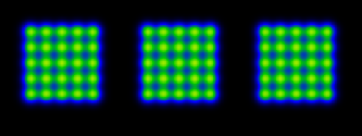
Example
|
region{
binary{ name = "InAs" }
array_x{ shift=20 num=5 }
array_y{ shift=20 num=5
}
array2_x{ shift=150 num=3
}
array2_y{ shift=150 num=3 }
repeat_profiles = 'other doping'
circle{
center{ x=100 y=100
}
radius = 30
}
doping{
gaussian2D{
name = B
conc=1e18 x=100 y=100 sigma_x=7 sigma_y=7 add=yes}
}
}
} |
For repeated structures which extend beyond the bounds of the simulation regions,
please make sure that
min and max
are large enough to also include objects which are partially outside of the simulation region.
Note: When
periodic{...}
is used, objects extending over an edge of the simulation region will not automatically be continued on the opposite side.
If such objects are present in a periodic simulation, for each periodic coordinate direction
(x, y or z), please
either define a repetition
(using the size of the simulation region as shift with
max = 1
and/or min =
1
as needed),
or extend an
already present repetition to the edge of the simulation region (by increasing
min and max
as needed).
Warning: Special care has to be taken
when using remove{}
or add = no
for doping{}/fixed charge/generation{}
in some repeated regions.
Namely, repeated
regions are created by sequentially creating multiple instances of a given
region at the different positions defined by the
array_*
and
array2_*
statements.
But the order in which these instances are created depends on
undocumented implementation details and thus may change from release to release.
For additive dopants/fixed charges/generation, or for repeated regions which do
not self-overlap,
the final structure and profiles do not depend on this
undocumented creation order and thus no problems will occur.
However, for
repeated regions which self-overlap (e.g. due to small region shifts),
using
remove{}
or add = no
results in the final structure and profiles being dependent
on that creation order and often being different from the user's intentions.
Therefore, in case of doubt, please visually inspect your structure and profiles
to avoid such issues.
} # region
} # structure
|