www.nextnano.com/documentation/tools/nextnano3/input_syntax/keywords/optical-absorption.html
Optical absorption
Detailed description about the Physics:
Absorption, Matrix elements, Inter-band transitions, Intra-band transitions.
A tutorial is available that describes this keyword:
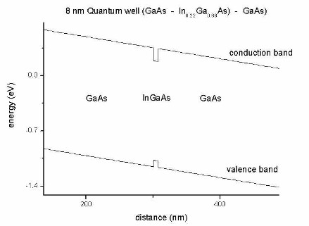
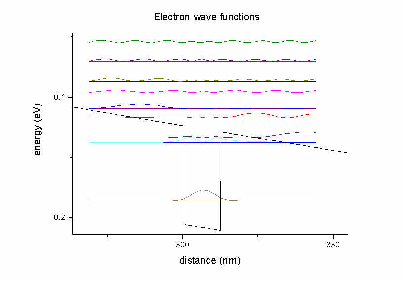
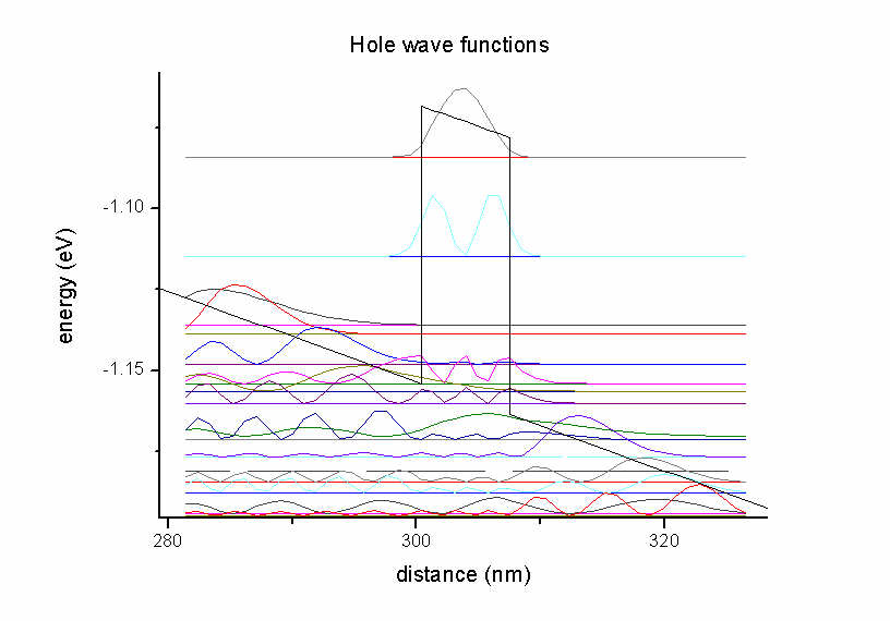
Optical absorption of an InGaAs quantum well
Here you can specify the options for the optical absorption.
This will be a 3-step approach:
- Step 1:
calculate-optics = no
Solve k.p and determine lowest and highest eigenvalue to specify
e-min-state and e-max-state in the second step.
- Step 2:
  calculate-optics = yes

  read-in-k-points = no
raw-potential-in = yes, raw-fermi-levels-in
	= yes, strain-calculation =
  raw-strain-in
- Step 3: Calculate optical absorption
  calculate-optics = yes

  read-in-k-points = yes
If one wants to repeat the calculation for another polarization, one only
needs to change the polarization vector and repeat step 3.
It is not necessary in this case to recalculate step 1 or step 2.
Step 3 also outputs the energy dispersion E(k||) = E(kx,ky).
!---------------------------------------------------------!

$optical-absorption
optional  !

 destination-directory
character
required  !

 calculate-optics
character
optional  !
flag: "yes"/"no"
kind-of-absorption
character
optional !
read-in-k-points
character
optional ! flag: "yes"/"no"
!
! if 'read-in-k-points = no' then specify
k point calculation !
2nd step
 num-quantum-cluster
integer
optional  !
 e-min-state
double
optional  ! [eV]
 e-max-state
double
optional  ! [eV]
!


!
 e-min-photon
double
optional  ! [eV]
 e-max-photon
double
optional  ! [eV]
 num-energy-steps
integer
optional  !

 smoothing-of-curve
character
optional ! "yes"/"no"
smoothing-damping-parameter
double
optional ! [eV] artificial damping parameter
for smoothing of absorption curve
 E-P
double
optional  ! [eV]  |<S|p|X>|^2

 polarization-vector-1
double_array  optional  ! x y z
 polarization-vector-2
double_array  optional  ! x y z
 magnitude-relation-1-2
double
optional  ! |E1|/|E2|

 phase
double
optional  ! E2 ->
exp(i*phase*Pi)*E2


!

 fermi_in_el
double
optional  ! [eV]
 fermi_in_hl
double
optional  ! [eV]
 device_thickness_in
double
optional  ! [m]
!

 k-space-symmetry
character
optional  !


!


!

 incident-light-along-direction
character
optional  ! x,y,z


!

 import-absorption-spectrum
character
optional ! "yes"/"no"
file-absorption-spectrum
character
optional !
!
import-reflectivity-spectrum character
optional ! flag: "yes"/"no"
file-reflectivity-spectrum
character
optional !
!
import-transmission-spectrum character
optional ! flag: "yes"/"no"
file-transmission-spectrum
character
optional !
!
import-solar-spectrum
character
optional ! flag: "yes"/"no"
file-solar-spectrum
character
optional !
!
number-of-suns
double
optional !
!
calculate-black-body-spectrum
character
optional ! flag: "yes"/"no"
$end_optical-absorption
optional !
!---------------------------------------------------------!
Syntax
destination-directory = optics1/
Directory for output and data files.
calculate-optics       =
yes


= no
Flag to distinguish between
- Step 1: For calculation of k.p wavefunctions for all k||
vectors), and
- Step 2 and Step 3: Reading in previously calculated k.p
wavefunctions for all k|| vectors (in order to save CPU time), and
then calculating the optical absorption.
e-min-photon
= 1.500      ! [eV]
lower boundary
for photon energy
e-max-photon           =
1.700      ! [eV]
num-energy-steps       =
1000
Number of energy steps between e-min-photon and
e-max-photon.
This number determines the resolution of the absorption curve alpha(E) where E
is the energy in units of [eV].
==> The number of energy grid points = num-energy-steps + 1
because the first grid point (e-min-photon) is also
included.
First step
kind-of-absorption     = interband-only


= intra-vb-only


= intra-cb-only


= intra-sg-only

'interband-only':
considers only interband transitions between holes and
electrons
heavy hole     <-->   Gamma band


light hole     <-->   Gamma band


split-off hole <-->   Gamma band

'intra-vb-only' :
heavy hole     <-->   light hole


heavy hole     <-->   split-off hole


light hole     <-->   split-off hole


heavy hole     <-->   heavy hole


light hole     <-->   light hole


split-off hole <-->   split-off hole

'intra-cb-only' :
Gamma band     <-->   Gamma band

'intra-sg-only' :
Gamma band     <-->   Gamma band


L band         <-->   L band


X band         <-->   X band


heavy hole     <-->   heavy hole


light hole     <-->   light hole


split-off hole <-->   split-off hole
read-in-k-points       =
yes


= no
Flag to distinguish between step 2 and 3.
Second step
If 'read-in-k-points = no' then specify k point
calculation. (These parameters will be ignored in Step 3.)
num-quantum-cluster = 1 !
(optional)
If this specifier is not present, the default value (num-quantum-cluster = 1)
is taken.
e-min-state
= -1.7      ! [eV]
lowest eigenvalue
e-max-state            =
0.3      ! [eV]
$quantum-model-electrons
 ...

 num-kp-parallel  =
  1700   ! STEP 2/3
  !
total number of k|| points for Brillouin zone
discretization
$quantum-model-holes
 ...

 num-kp-parallel  =
  1700   ! STEP 2/3
  !
total number of k|| points for Brillouin zone
discretization
However, internally the code modifies this number according to the following
algorithm:
- number of k points in positive x direction (without Gamma point):
N_kx
- number of k points in positive y direction (without Gamma point):
N_ky
= N_kx
==> Thus the actual, total number of k|| points
is:
total_number_of_k||
= (2 * N_kx + 1) * (2 * N_ky + 1)
In this example (num-kp-parallel = 1700):
- N_kx = N_ky = 20
==> total_number_of_k|| = 41 * 41 = 1681
Third step
'read-in-k-points = yes' to read in k points, calculate
and output optical absorption.
smoothing-of-curve
= yes     !
(default)
= no      !

smoothing-damping-parameter = 0.5e-3  ! [eV]
Lorentzian.
The artificial parameter for smoothing of absorption curve is
smoothing-damping-parameter. It is usually denoted as Gamma and is the
Full Width at Half Maximum (FWHM).
  absorption_NoSmoothingV = absorptionV

  absorptionV = 0.0

  DO  i=1,num-energy-steps+1 ! Loop over all energy grid points E(i) and determine
absorption alpha(i)=alpha(E).

   DO j=1,num-energy-steps+1 ! This loop is essentially an integration over energy dE.


    E_weight = (Lorentzian( E_gridV(j),
  E_gridV(i), smoothing-damping-parameter )
- &


Lorentzian( E_gridV(j),
 - E_gridV(i), smoothing-damping-parameter )
) * DeltaEnergy


    absorptionV(i) = absorptionV(i) + absorption_NoSmoothingV(j) * E_weight


   END DO

  END DO
Lorentzian lineshape
   FUNCTION Lorentzian (E,E0,Gamma)


Lorentzian = 1 / pi * alpha / ( (E - E0)2
+ alpha2
)


            alpha
is the scale parameter 'Lorentzian half-width': Half Width at Half Maximum (HWHM)
            alpha = Gamma
/ 2 = smoothing-damping-parameter / 2


   DeltaEnergy = (e-max-photon
- e-min-photon ) / (num-energy-steps)


E_gridV = [eV]
DO i=1,num-energy-steps+1
E_gridV(i) =
e-min-photon + (i-1) * DeltaEnergy
END DO
The following specifiers are only used for the k.p optical
absorption algorithm but not for the simple intersubband transition algorithm.
E_P
= 22.0
! [eV]

E_P
is Kane's matrix element EP = | < S | p | X > |2.
It
should be around 20 eV and depends on the material.
The E_P [eV] parameter is given in the database by the specifier
8x8kp-parameters.
E_P can be converted into the P paramter by the following equation:
EP = 2m0/hbar2 * P2
In our model the E_P parameter is only relevant for interband
transitions. It enters into the matrix element prefector (matrix_element_prefac)
which is described in Section "1.1.1 Inter-band transitions" of the
documentation:
Absorption, Matrix elements, Inter-band transitions, Intra-band transitions.
E_P has the same value for all materials in this implementation. In
principle it could have been read in from the database rather than specifying it
within the keyword
$optical-absorption.
polarization-vector-1  = 1.0  0.0  0.0

polarization-vector-2  = 0.0  1.0  0.0

x y z
coordinates (in simulation system) for first/second in-plane vector
Example:
- 1D well, inter-band
polarization-vector-1  = 1.0  0.0  0.0

polarization-vector-2  = 0.0  1.0  0.0

  magnitude-relation-1-2 = 1.0
- 1D well, intra-band
polarization-vector-1  = 0.0  0.0
  1.0

polarization-vector-2  = 0.0  0.0  1.0

  magnitude-relation-1-2 = 0.0
Note: Intraband absorption only for z-polarized light.
How to specify x-polarized light:
 polarization-vector-1  = 0.0 1.0 0.0
  !
x y z coordinates (in simulation system) for first in-plane vector
 polarization-vector-2  = 1.0 0.0 0.0
  !
 magnitude-relation-1-2 = 0.0
! |E1|/|E2|
(In this case, polarization-vector-1 is ignored as
|E1| is set to be zero.)
 polarization-vector-1  = 1.0 0.0 0.0
  !
x y z coordinates (in simulation system) for first in-plane vector
 polarization-vector-2  = 0.0 0.0 1.0
  !
 magnitude-relation-1-2 = 0.0
! |E1|/|E2|
(In this case, polarization-vector-1 is ignored as
|E1| is set to be zero.)
 polarization-vector-1  = 1.0 0.0 0.0
  !
x y z coordinates (in simulation system) for first in-plane vector
 polarization-vector-2  = 0.0 0.0 1.0
  !
 magnitude-relation-1-2 = 1.0
! |E1|/|E2|
(In this case, polarization-vector-1 is not ignored as
|E1|=|E2|.)
magnitude-relation-1-2 = 1.0
relation of magnitudes |E1|/|E2|
phase
= 0.5
phase: E2-> exp(i*phase*Pi)*E2
fermi_in_el
= 0.0     ! [eV]
optional input for Fermi level of electrons (default: calculated Fermi
level)
fermi_in_hl
= 0.0     ! [eV]
optional input for Fermi level of holes
(default: calculated Fermi level)
device_thickness_in = 1e-6 ! [m]
optional input of device thickness for normalization of absorption
k-space-symmetry       =
default    !
(default)
                       =
none       !

                       =
four-fold  !
By default, the appropriate symmetry is chosen taking into account any crystal
rotations with respect to the simulation axes, as well as nonsymmetric strains.
Results:
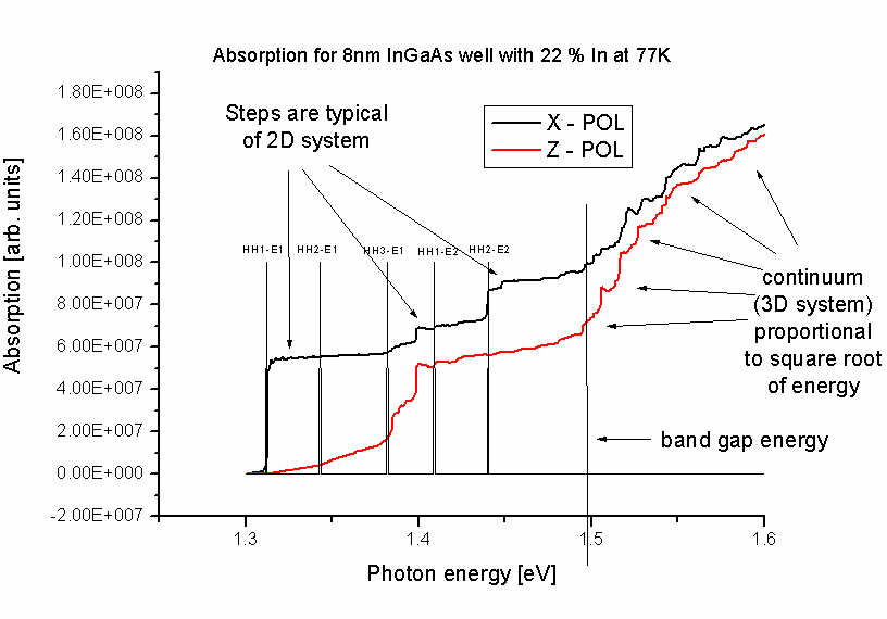
The units of the optical absorption are [1/m] and not "arbitrary units" as
indicated in the figure.
- The electric susceptibility tensor is contained in the file
susceptibility_tensor.dat:
chi11re  chi11im  chi22re  chi22im
chi33re  chi33im  chi12re  chi12im
chi13re  chi13im  chi23re  chi23im
re: real part,
im: imaginary part
The relevant part for the absorption is
only the imaginary part.
- In step 3, for each electron (
el) and for each hole
(hl) eigenvalue (i.e. ev00*), the
energy dispersion E(kx,ky) is written out to the
following files:
optics/kp_optics_el_dispersionAVS2D_ev001.fld, *.coord,
	*.dat

	...

	optics/kp_optics_hl_dispersionAVS2D_ev001.fld, *.coord, *.dat

	...
The format of the files is compatible to the AVS/Express software.
The following figure shows the energy dispersion E(kx,ky)
of the highest hole eigenstate (ground state).
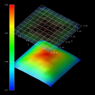
The units of the k|| space grid coordinates kx
and ky are [1/Angstrom] and the energy units are [eV].
The files
- el_dispersion_100.dat

	- el_dispersion_110.dat

	- hl_dispersion_100.dat

	- hl_dispersion_110.dat
show the same data but with slices along the [10] (i.e. k||=(kx,ky=0))
and [11] (i.e. kx=ky) directions in k||
space.
Here all electron and all hole eigenvalues are contained in one file,
respectively.
Restrictions
- Only Dirichlet boundary conditions are supported so far.
- Step 2 and step 3 only work if
 raw-potential-in =
	yes
.
Solar cells
The following flags are useful for solar cell simulations (photovoltaics).
 incident-light-along-direction =  x          !
incident light along  x direction


=  y          !
incident light along  y direction


=  z          !
incident light along  z direction


= -x          !
incident light along -x direction


= -y          !
incident light along -y direction


= -z          !
incident light along -z direction
In a 1D simulation, this specifier is optional. For 2D, and 3D, a
direction must be specified.
Solar spectrum
For a solar cell simulation, one has to read in a solar spectrum, e.g. AM
1.5, or AM 1.0 (AM = air mass).
They can be obtained from NREL website, e.g. ASTM-E490:
https://www.nrel.gov/grid/solar-resource/spectra-astm-e490.html
(AMST = American Society for Testing and Materials)
  import-solar-spectrum
= yes


   = no


!file-solar-spectrum
= H:\solar_cells\ASTMG173_AM10.dat  !
AM 1.0 spectrum (extraterrestrial)
!file-solar-spectrum
= H:\solar_cells\ASTMG173_AM15.dat  !
 file-solar-spectrum
= H:\solar_cells\ASTMG173_AM15G.dat !
[nm] and [W/m^2*nm^-1].
   wavelength[nm]    AM1.5[W/m^2*nm^-1]

   ...
...
  number-of-suns
=    1.0

!    1   sun


=    2.5

!    2.5 suns


=   10.0

!   10   suns


= 1000.0

! 1000   suns
To increase the power of the solar spectrum in order to model
concentrator solar cells.
Absorption coefficient
 import-absorption-spectrum      =
yes


   = no


 file-absorption-spectrum        =
AbsorptionCoefficient_GaAs_300K.dat
The file must consist of two columns (wavelength and absorption
coefficient), the units are [nm] and [1/cm].
   wavelength[nm]    absorption[1/cm]

   ...
...
Reflection coefficient
Fraction of incident photons that are reflected from surface for a particular
wavelength.
 import-reflectivity-spectrum    =
yes


   = no


 file-reflectivity-spectrum      =
ReflectionCoefficient_GaAs_300K.dat
The file must consist of two columns (wavelength and reflection
coefficient), the units are [nm] and [].
   wavelength[nm]    reflectivity[]

   ...
...
Transmission coefficient
Fraction of incident photons that are transmitted through the device for a
particular wavelength (relevant for very thin devices).
  import-transmission-spectrum    =
yes


   = no


 file-transmission-spectrum      =
ReflectionCoefficient_GaAs_300K.dat
The file must consist of two columns (wavelength and transmission
coefficient), the units are [nm] and [].
   wavelength[nm]    transmission[]

   ...
...
Black body spectrum
  calculate-black-body-spectrum =
yes


 = no
Calculates black body spectrum according to
Planck's
law, e.g. to
compare the solar spectrum to the spectrum of a black body at T = 5778 K.
- The spectral energy density
- the spectral radiance (which is emitted per m2 and
per unit solid angle sr (sr = steradian)) and
- the spectral irradiance (which is received per m2)
is calculated.
Note: spectral irradiance = spectral radiance * pi
spectral energy density =
spectral radiance * 4pi/c
There are several output files, i.e. output with respect to
- wavelength lambda in units of [m].
	BlackBody_SpectralEnergyDensity_wavelength.dat

  Wavelength[nm]
	SpectralEnergyDensity[kJ/m^3/m]
	BlackBody_SpectralRadiance_wavelength.dat

  Wavelength[nm]
	SpectralRadiance[kW/m^2/nm/sr]
BlackBody_SpectralIrradiance_wavelength.dat

  Wavelength[nm]
	SpectralIrradiance[kW/m^2/nm]
- angular frequency w = 2pi v in units of [1/s].
	BlackBody_SpectralEnergyDensity_angular_frequency.dat

  AngularFrequency_omega[10^15/s]
	SpectralEnergyDensity[10^-15J/m^3/s^-1]
	BlackBody_SpectralRadiance_angular_frequency.dat

	  AngularFrequency_omega[10^15/s]
	SpectralRadiance[10^-12W/m^2/s^-1/sr]
BlackBody_SpectralIrradiance_angular_frequency.dat
  AngularFrequency_omega[10^15/s]
	SpectralIrradiance[10^-12W/m^2/s^-1]
- frequency v in units of [Hz].
		BlackBody_SpectralEnergyDensity_frequency.dat

  Frequency[THz]
	SpectralEnergyDensity[10^-15J/m^3/Hz]
	BlackBody_SpectralRadiance_frequency.dat

	  Frequency[THz]
	SpectralRadiance[10^-12W/m^2/sr]
		BlackBody_SpectralIrradiance_frequency.dat

  Frequency[THz]
	SpectralIrradiance[10^-12W/m^2/Hz]
- photon energy E = h v in units of [eV].
		BlackBody_SpectralEnergyDensity_energy.dat

  AngularFrequency_omega[10^15/s]
	SpectralEnergyDensity[kJ/m^3/eV]
	BlackBody_SpectralRadiance_energy.dat

	  AngularFrequency_omega[10^15/s]
		SpectralRadiance[kW/m^2/eV/sr]
		BlackBody_SpectralIrradiance_energy.dat

  AngularFrequency_omega[10^15/s]
	SpectralIrradiance[kW/m^2/eV]
The file BlackBody_Info.txt contains some additional information
about the calculated black body spectrum.
Solar cell output
All output is twofold:
- one is with respect to wavelength in units of [nm]
- one is with respect to photon energy in units of [eV] (indicated by
_eV*.dat)
optics/Absorption_coefficient.dat
(as read in from file but now in units of [1/m])
optics/Absorption_coefficient_interpolated.dat
optics/Reflectivity.dat
optics/Reflectivity_interpolated.dat
optics/Transmission.dat
optics/Transmission_interpolated.dat
optics/SolarSpectralIrradiance_sun0001.dat
optics/PhotonFlux_sun0001.dat
optics/PhotonFlux_BandGap_eV_sun0001.dat
optics/PhotoCurrent_BandGap_eV_sun0001.dat
	optics/SpectralResponse_sun0001.dat
	external and internal spectral response

	optics/QuantumEfficiency_sun0001.dat
	external and internal quantum efficiency

	optics/GenerationRateLight_AVS_sun0001.fld      2D
	plots GenerationRate(x,lambda) and  GenerationRate(x,E)

	optics/GenerationRateLight_sun0001.dat
	1D plot  GenerationRate(x)

	optics/GenerationRate_eV_sun0001.dat
	1D plot  GenerationRate(E)  (E=energy)

	optics/GenerationRate_Wavelength_sun0001.dat    1D plot
	GenerationRate(lambda)
current/IV_characteristics_new.dat


	voltage[V]  current[A/m^2] ... power[W/m^2] powersolar[W/m^2]
	efficiency[%]
	 ****************************************************************************************

 Solar cell results

 ****************************************************************************************

 short-circuit current:       I_sc     =       281.473346 [A/m^2]                  (photo current: It increases with smaller band gap.)

 open-circuit voltage:        U_oc     =  -1.012500 [V]                           (U_oc <= built-in potential ~ band gap)

 current at maximum power:    I_max   =       273.089897 [A/m^2]

 voltage at maximum power:    U_max   =  -0.925000 [V]

 maximum power output:        P_max   = U_max * I_max =      -252.608155 [W/m^2] (condition for maximum power output: dP/dV = 0)

 maximum extracted power:     P_solar = - P_max           =  252.608155 [W/m^2]

 incident power:              P_in     =   0.000000 [W/m^2]

 ideal conversion efficiency: eta     = P_max / P_in  =         Infinity %

 fill factor:                               FF      =   0.886370

 In practice, a good fill factor is around 0.8.

 All these results are approximations.

 They are only correct if a lot of voltage steps have been used (i.e. a high resolution).

 ****************************************************************************************
|